Introduction
In this article we will look at how to simulate a spherical wave produced from point source .
Wave Propagation and Spreading Loss
According to wave theory a point source produces a spherical wave in an ideal isotropic (uniform) medium such as air.
If wave propagates at velocity $t$,time taken for the wave to propagate from point A to B is given by
$\displaystyle \tau=\frac{d(A,B)}{v}$
If $x(t)$ is signal associated with the source,then the signal y(t) at the listening point can be expressed as
$\displaystyle y(t) = \alpha * x(t - \tau)$
Thus these is a phase delay between the signal observed at source and destination locations.
This can be easily simulated by delay line.
In digital domain the analog wave is sampled at frquency $F_{s}$.Thus a time duration of $\tau$ sec will correspond to $\tau*F_{s}$ samples.
Thus signal observed at listening point is time delay version of signal associated with the source
$ \displaystyle y[n] = \alpha * x [ n- \tau N] = \alpha x [ n - \beta]$
where $\beta$ can be fractional.
In the previous article `` we saw how to implement fractional delays.The same function will be used here to introduce a delay corresponding to wave propagation time between points A and B.
        def propagation_delay(self,source):
            """ the function completes the sample delay of source signal

            Parameters
            -----------
            source - numpy array ,shape (Nxdimension)
                     source location

            Returns
            ----------
            diff - numpy array ,shape (Nx1)
                   distance of receiver to source

            """
            diff1=[]
            for i in range(len(source)):
                diff1.append(Utils.distance(self.position,source[i]))
            diff1=np.array(diff1)
            return diff1

        def sample_delay(self,source):
            """" computes the sample delay of source signal observed
            at receiver

            Parameters
            -----------
            source - numpy array ,shape (Nxdimension)
                     source location

            Returns
            ----------
            delay - numpy array ,shape (Nx1)
                    sample delay corresponding to propagationtime

            """
            dist=propagation_delay(source)
            delay=dist*self.Fs/self.velocity
            return delay
Wave energy is conserved as it propagates through the air. In a spherical pressure wave of radius $ r$ , the energy of the wavefront is spread out over the spherical surface area $ 4\pi r^2$ . Therefore, the energy per unit area of an expanding spherical pressure wave decreases as $ 1/r^2$ . This is called spherical spreading loss.
Energy is proportional to amplitude squared, an inverse square law for energy translates to a $ 1/r$ decay law for amplitude.
Thus the amplitude of wave reduces by a factor of $1/r$ for a traversal distance of $r$
        def propagation_loss(self,source):
            """ the function completes the spreading loss of signal
            from source to present location

            Parameters
            -----------
            source - numpy array ,shape (Nxdimension)
                     source location

            Returns
            ----------
            loss - numpy array ,shape (Nx1)
                   spreading propagation loss

            """
            dist=self.propagation_delay(source)
            loss=1.0/dist
            return loss
Thus the wave at receiver can be simulated wrt to wave associated with source by introducing a time delay and attenucation corresponding to distance travelled
        def run(source,signal):
            """" simulates the signal at the wave receiver

            Parameters
            -----------
            source - numpy array ,shape (Nxdimension)
                     source location

            signal - numpy array,shape (1xN)
                     signal associated with source

            Returns
            ----------
            delay - numpy array ,shape (Nx1)
                    wave at the receiver due to multiple sources

            """

            delay=self.sample_delay(source)
            loss=self.propagation_loss(source)
            signal=Utils.fdelay(signal,delay)
            signal=signal1*loss*absorbtion


            for i in range(len(source)):
                signal[i]=Utils.addNoise(signal[i],self.noise)
                seed=int(np.random.uniform(0,1)*10000);
                np.random.seed(seed)

            signal=np.sum(signal)


            if self.phase_shift!=0:
                signal=Utils.phase_sift(signal,self.phase_shift)

            return signal
For a modular implementation we describe WaveSource and WaveSink classes
that encapsulate the properties of wave source and receiver.
The WaveSource contains simply the location of source,propagation properties of wave and source signal
class WaveSource(object):
    def __init__(self,position,attenuation,phase,velocity,carrier,Fs):
        self.position=np.array(position)
        self.attenuation=attenuation
        self.phase=phase
        self.carrier=carrier

        #generate default modulated sinusiodal waveform
        to=100;
        t1=100+(100*Fs/3000);
        l=1000*Fs/3000;

        waveform=4*Utils.sinepulse(l,to,t1,carrier,Fs)

        self.signal=waveform

""" The Wave souce is initialized as follows """'

    #souce signal properties
    Fs=48000
    carrier=1000
    velocity=300

    #souce location
    source=[[5,3],[5,-3],[-5,3],[5,17],[15,3]]
    phase =[0,math.pi,math.pi,math.pi,math.pi]
    attenuation=[1,0.5,0.5,0.5,0.5]

    sources=[]
    for i in range(len(source)):
        s=WaveSource(source[i],attenuation[i],phase[i],velocity,carrier,Fs)
        sources.append(s)
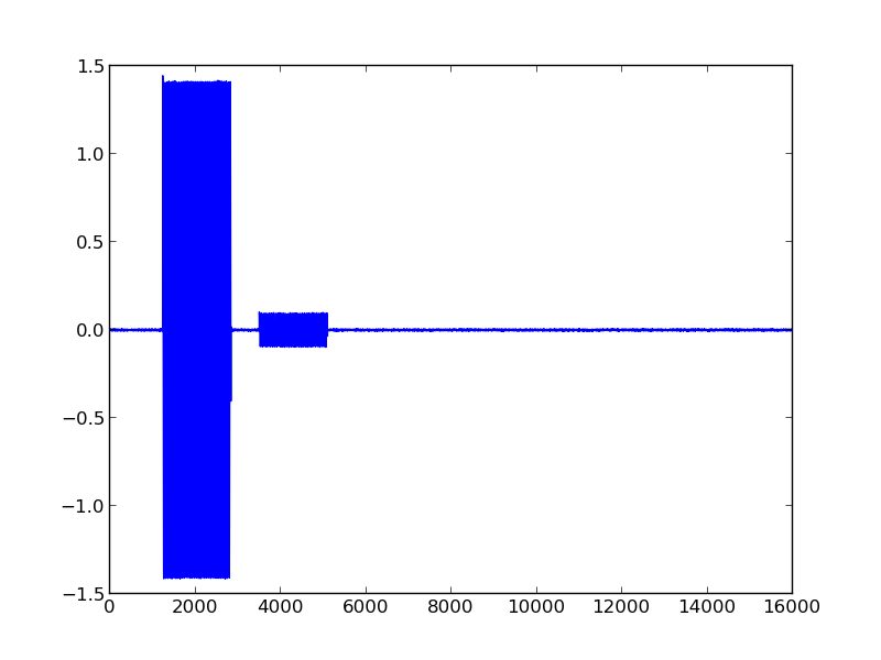
The WaveSink compute the propagation time.sample delay,propagation loss and performs computation on each WaveSink object to generate a wave output corresponding to each source.Then it adds all outputs dues to individual sources to get a combined output at the receiver due to all the sources
    receivers=[10,10]
    sink=WaveSink(receivers,Fs,velocity,0,1.0,0.001)
    signals=sink.run(sources)

Code
The code for the same can be found in file WaveSink.py and WaveSouce.py in pyVision github repository
To run the code clone the entire pyVision github repository
The code to generate the waveform can be executed by going to the pySignalProc directory of the repository and executing WaveSink.py file
- Github Repo Link
- Links to files WaveSink.py and WaveSource.py