Introduction
In this article we look at Approximation of Piecewise Polynomial Using Wavelets
Wavelet Approximation of polynomials
In many application,one needs to approximate a signal using scaling function ie using projection on $V_{m}$ subspace.
The support of a function is the set of points where the function is not zero-valued,The support of $\phi(t),\psi(t)$ which is defined over unit interval is 1
The basic analysis starts with considering a set of monomials ${1,t,t^2,\ldots,t^{k} }$ and asking the question till what degree $k$ can these be reproduced exactly using the scaling function.
Let us assume that $t^{p}$ can be represented exactly using the scaling function $t^{p} = \sum_{k} d_{k} \phi(t - k)$
Orthonormality of basis function impies
$d_{k} = \int t^{p} \phi(t -k ) dt$
To achieve this the scaling function should possess a certain properties which is dependent on the filter coefficients .
Restrictions on scaling and wavelet function
This assumption will impose certain restriction on the scaling and wavelet function
$\int t^{p} \psi(t) dt = \int \sum_{k} d_{k} \phi(t - k)\psi(t) dt = \sum_{k} d_{k} \int \phi(t - k)\psi(t) dt $
$\psi(t) ,\phi(t)$ are orthogonal ,meaning that $\phi(t)$ is capable of expressing polynomials upto degree $p$ exactly.
The projection of $t^{p} $ on $W_{m}$ subspace is 0. The projection of $t^{p} $ on $W_{m}$ subspace will not be zero only when it cannot be expressed completely by the scaling function.
if $p=0$,The condition implies
$\int \psi(t) dt =0$
Indicating that a constant function can always be expressed completely by scaling function.
we know that
$\psi(t) = \sum_{k} g[k] \phi(2t - k)$
$\phi(t) = \sum_{k} h[k] \phi(2t -k )$
We will use a result here which will be derived in later articles
$\int \psi(t) \phi(t) dt =0$ for this to hold true
$g[k]=(-1)^{N-k-1}h(N-k-1)$ and
$\psi(t) = \sum_{k} (-1)^{N-k-1}h(N-k-1) \phi(2t + k -N+1)$
for even N
$g[k]=(-1)^{k}h(N-k-1)$
$\int \sum_{k} (-1)^{N-k-1}h(N-k-1) \phi(2t + k -N+1) dt=0$
$\sum_{k} (-1)^{k} h(k) \int \phi(y) dy=0$
Vanishing Momemnt Constraint on wavelet filter coefficients
Zero order vanishing moment constraint $\sum_{k} (-1)^{k} h(k) =0$
pth order vanishing moment constraint $\sum_{k} (-1)^{k} k^{p}h(k) =0$
These vanishing moment constraint imposed on scaling and wavelet function help solve for the filter coefficients.
Projection of polynomials on subspace defined by Wavelets
Wavelet function $\psi(t)$ having N vanishing moments will kill polynomial upto degree $p-1$
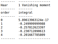
Let us look at a Haar wavelets function and projection of increasing order of polynomials on Haar wavelet basis.Haar wavelet has 1 vanishing moment.
Thus it can only kill polynomial of order 1 or constant function
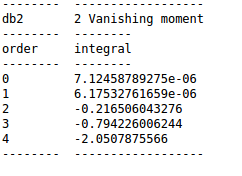
Daubechies -2 wavelet has vanishing moment of 2 ,Thus it can kill polynomial upto degree of 2 A constant and linear function.
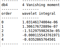
Daubechies -4 has vanishing moment of 4 ,Thus it can kill polynomials upto a degree of 3
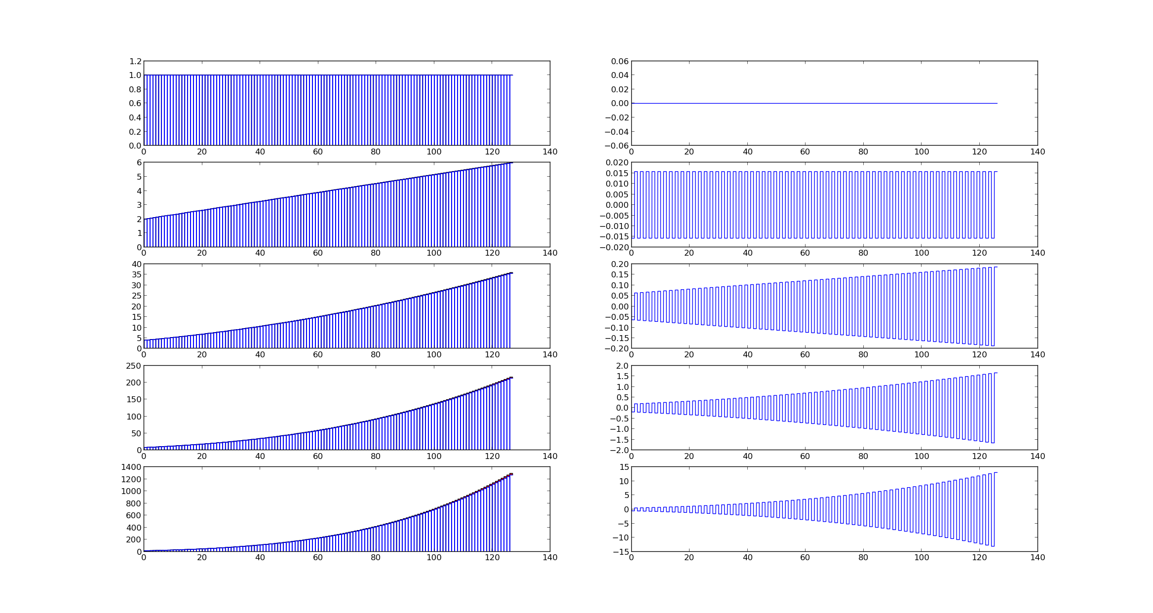
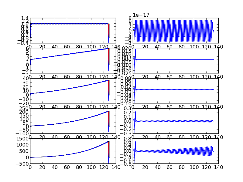
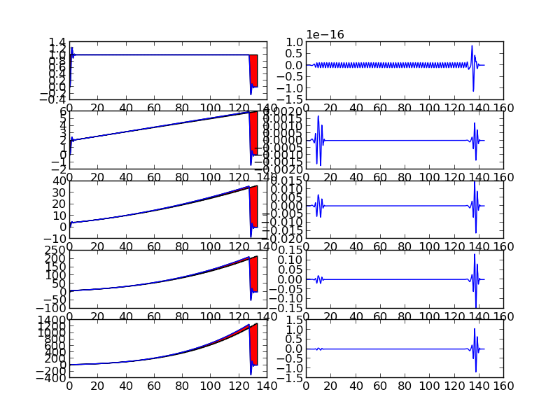
What this means is that projection on $W_{o}$ subspace is zero.Wavelet coefficients will have low magnitude .Typically threshold should be less than $1^{-7}$.This will imply signal can be reconstructed from the projection on $V_{0}$ subspace to a great degree of accuracy
We can see the projection on the $V_{0}$ and $W_{0}$ subspace in the below figures
Projection of Piecewise polynomials on subspace defined by Wavelets
It is important to note that it is sufficient that function behaves like a polynomial of degree $k$ over support of function for it to be approximated by scaling function.
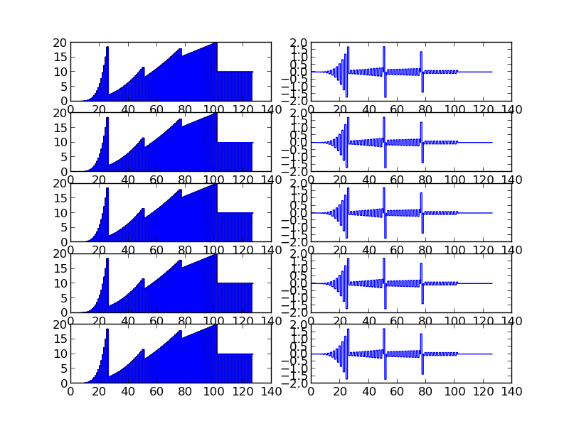
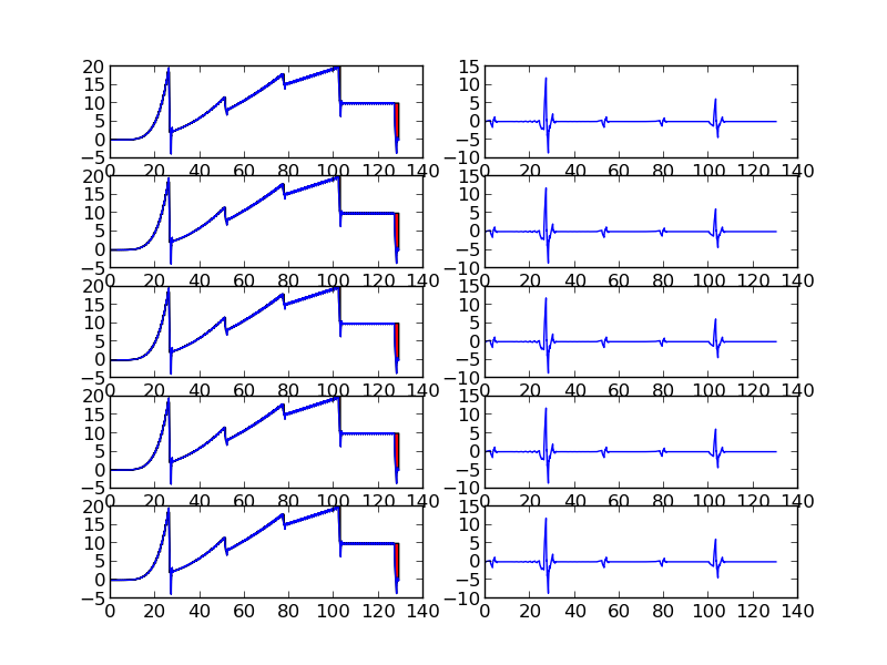
Below figures show piecewise polynomials and projection on $V_{0}$ and $W_{0}$ subspace
We can see that piece-wise polynomials of degree $p$ within the support of wavelet functions with vanishing moment $p$ have zero wavelet coefficients except at points of discontinuity
Code
The function plotwaveletProjection plots the projection of signal onto the $V_{m}$ and $W_{m}$ subspace
def plotWaveletProjection(x,coeff,w,level=1,mode=0):
""" function plots the projection of signal on the scaling and wavelet functions subspace
Parameters
-----------
x : numpy-array,
The input signal
coeff : numpy=-array
The wavelet or scaling coefficient
w : pywt.Wavelet
wavelet object
level : integer
decomposition level
mode : integer
scaling or wavelet coefficient
Returns
--------
out : numpy-tuple
(time,reconstruction,signal)
"""
#generate the scaling and wavelet functions
s1,w1,t2=w.wavefun(level=20)
#setup 1D interpolating function for scaling and wavelet functions
wavelet=interpolate.interp1d(t2, w1)
scaling=interpolate.interp1d(t2, s1)
time=[]
sig=[]
s1=np.array(s1,float)
#compute the dydactic scale
l=2**level
#find the support
end1=math.floor(t2[len(t2)-1])
d=abs(float(len(coeff))*float(l)-len(x))
d=int(d)
#range over each element of coefficient
for i in range(len(coeff)-1):
#define the interpolation points
t=np.linspace(l*i,l*i+l*end1,l*end1*(len(x)));
t1=np.linspace(0,end1,end1*(len(x))*l);
#multiply the coefficient value with scaling or interpolation function
if mode==0:
val=coeff[i]*scaling(t1)
else:
val=coeff[i]*wavelet(t1)
ratio=end1
#compute the translation
inc=len(t)/ratio
if i==0:
sig=np.append(sig,val)
time=np.append(time,t)
else:
#compute the incremental sum of signals
v1=val[0:len(t)-inc]
if inc < len(t):
v2=val[len(t)-inc:len(t)]
sig[i*inc:i*inc+len(t)]=sig[i*inc:i*inc+len(t)]+v1
sig=np.append(sig,v2)
time=np.append(time,np.linspace(l*i+l*end1-l,l*i+l*end1,inc))
else:
sig=np.append(sig,val)
time=np.append(time,t)
#flatten the arrays
sig=np.array(sig).flatten()
time=np.array(time).flatten().ravel()
#scale the values due to didactic decomposition
sig=sig/(math.sqrt(2)**level)
#upsamples the value of signal
x=np.repeat(x,len(sig)/len(x))
#return the signals,which can be plotted
return time,sig,x
A class called “PiecewiseContinuous “ encapsulates all the methods that define a piece-wise continuous function.The function is modified version of the function from sagemath library
 # piecewise function
def f1(x):return 10
def f2(x):return 5*x
def f3(x):return 2*(x)**2
def f4(x):return (x)**3+(x)**2
def f5(x):return 20*((x)**5)

f = Piecewise([[(0,1),f5],[(1,2),f4],[(2,3),f3],[(3,4),f2],[(4,5),f1]])

f(1) will give the value the value of piecewise function at 1
All the plots and results presented in the article can be generated by running the wavelet4.py files
Files
The code can be found in pyVision github repository
- pyVision/pySignalProc/tutorials/wavelet4.py
- pyVision/pySignalProc/wavelet/pywtUtils.py