Haar Wavelet Filter Bank

Introduction

In this article we will look at discrete time signal processing using wavelets,more specificially we will look at the concept of Haar Filterbank

In the previous article Haar Wavelets we saw the basics of harr wavelet and how a continuous time/discrete time signal can be expressed as sum of projection onto sub-spaces defined by wavelet and scaling function.

Analysis/Decomposition Filters

We saw that if we assume that the sampled signal is a projection onto subspace $V_{0}$ then using Harr scaling and wavelet function we can express the signal in terms of its projection on the subspaces $V_{-1} $ and $ W_{0}$

The process of expressing the signal by projecting on to subspaces of lower resolution is called as wavelet decomposition.

At each decomposition stage we project signal in subspace $V_{m}$ to subspaces $V_{m-1}$ and $W_{m}$ which are defined by scaling and wavelet functions.

We can see that once a we consider a projection on $V_{m}$ subspace we are dealing with a discrete time sequence.Let sequence be represented by $x[n]$

The projection of signal from $V_{m}$ to $V_{m-1}$ using haar scaling function can be

$\displaystyle y[n] = \frac{1}{\sqrt2} x[2n] + x[2n+1]$

Let $y_{o}[n]= \frac{1}{\sqrt2} x[n] + x[n+1]$

$\displaystyle _{l}[n] = y_{o}[2n]$

The projection operation can be obtained by performing following steps

• Apply discrete time filter $h_{l}[n]$ to discrete time signal which represents the projection of signal onto $V_{m}$ subspace
• Downsample the signal by a factor of 2 to get the projection on $V_{m-1}$ subspace

The projection of signal from $V_{m}$ to $W_{m}$ subspace using haar wavelet function can be expressed as

$\displaystyle y[n] = \frac{1}{\sqrt2} x[2n] - x[2n+1]$

Let $y_{o}[n]= \frac{1}{\sqrt2} x[n] - x[n+1]$

$\displaystyle y_{h}[n] = y_{o}[2n]$

The projection operation can be obtained by performing following steps

• Apply discrete time filter $h_{u}[n]$ to discrete time signal which represents the projection of signal onto $V_{m}$ subspace
• Downsample the signal by a factor of 2 to get the projection on $W_{m}$ subspace

$\displaystyle h_{l}[n]= \frac{1}{\sqrt2} [ 1 , 1 ] $ or $h_{l}[z] = \frac{1}{\sqrt2}[ 1 + z^{-1}]$

$\displaystyle h_{u}[n]= \frac{1}{\sqrt2} [- 1 , 1 ] $ or $h_{u}[z] = \frac{1}{\sqrt2}[ 1- z^{-1}]$

$h_{l}[n]$ computes the average of neighborhood samples acting as a low pass filter.The filter that projects onto subspace $V_{m-1}$ is called as low pass decomposition filter or low pass analysis filter

$h_{h}[n]$ computes the difference between neighborhood samples acting as a high pass filter.The filter that projects onto subspace $W_{m}$ is called as high pass pass decomposition filter or high pass analysis filter

The projection operation can be represented graphically as

Reconstruction/Synthesis Filters

Given projection on signal on $V_{m-1}$ and $W_{m}$,given

$\displaystyle y_{l}[n] = \frac{1}{\sqrt2} x[2n] + x[2n+1]$

$\displaystyle y_{h}[n] = \frac{1}{\sqrt2} x[2n] - x[2n+1]$

we can see that $\displaystyle x_{1}[n]=x[2n] = \frac{1}{\sqrt2} [y_{l}[n] + y_{h}[n] ]$

$\displaystyle x_{1}[n]=x[2n+1] = \frac{1}{\sqrt2} [y_{l}[n] - y_{h}[n] ]$

To get $x[n]$ we need to place samples of $x_{1}[n]$ are even integer location and $x_{2}[n] $ at odd integer location of $x[n]$

As example if $x_{1}[n]={1,2,3,4} $ and $x_{2}[n]={5,6,7,8}$ the desired sequence is $x[n]={1,5,2,6,3,7,4,8}$

This can be accomplished by first upsampling both the signals This will create a sequence new sequences $x_{1}[n],x_{2}[n]$ with zeros at odd integer locations

${1, 0 ,2 ,0, 3 ,0 4, 0, }$ and ${5, 0 ,6 ,0, 7 ,0 8, 0, }$

no we delay $x_{2}[n]$ ,this will lead to sequence with zeros at even integer locations

$\displaystyle {0,5, 0 ,6 ,0, 7 ,0 ,8}$ $\displaystyle {1, 0 ,2 ,0, 3 ,0 ,4, 0, }$

and adding both these signals will give us desired $x[n]$

$\displaystyle {1,5,2,6,3,7,4,8}$

This can be graphically represented as

We can as well upsample the original signals and then perform addition and subtraction and get the same result.

The equivalent block diagram can be expressed as

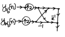
$\displaystyle x_{1}[n] = \frac{1}{\sqrt2} [y_{l}[\frac{n}{2}] + y_{h}[\frac{n}{2}] ]$

$\displaystyle x_{2}[n] = \frac{1}{\sqrt2} [y_{l}[\frac{n}{2}] - y_{h}[\frac{n}{2}] ]$

$\displaystyle x[n] = x_{1}[n] + x_{2}[n-1]$

The delay element can be shifted to the source

$\displaystyle x[n] = \frac{1}{\sqrt2} [y_{l}[\frac{n}{2}] + y_{h}[\frac{n}{2}] ]+ [y_{l}[\frac{n-1}{2}] - y_{h}[\frac{n-1}{2}] ]$

$\displaystyle x[n] = \frac{1}{\sqrt2} [y_{l}[\frac{n}{2}] + y_{l}[\frac{n-1}{2}] ]+ [y_{h}[\frac{n}{2}] - y_{h}[\frac{n-1}{2}] ]$

$\displaystyle x[n] = y_{l}[\frac{n}{2}] * h_{r,l}[n]+y_{h}[\frac{n}{2}] *h_{r,h}[n]$

where $\displaystyle h_{r,l}[n]= \frac{1}{\sqrt2} [ \delta[n] + \delta[n-1] ]$ is called low pass reconstruction/synthesis filter

$\displaystyle h_{r,h}[n]= \frac{1}{\sqrt2} [ \delta[n] - \delta[n-1] ]$ is called high pass reconstruction/synthesis filter

$\displaystyle h_{r,l}[n]= \frac{1}{\sqrt2} [ 1, 1] $

$\displaystyle h_{r,l}[n]= \frac{1}{\sqrt2} [ 1, -1] $

Thus we can see that we can recover the decomposed signal using above synthesis process

Haar Filter Bank

The entire process can be graphically represented as

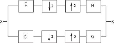
Let us look at what the analysis and synthesis filters are doing

Analysis of Decomposition filter

The decomposition filter coefficients are given by

$\displaystyle h_{d,l}[n]= \frac{1}{\sqrt2} [ 1 , 1 ] $ or $h_{l}[z] = \frac{1}{\sqrt2}[ 1 + z^{-1}]$

$\displaystyle h_{d,u}[n]= \frac{1}{\sqrt2} [- 1 , 1 ] $ or $h_{u}[z] = \frac{1}{\sqrt2}[ 1- z^{-1}]$

The Haar decomposition process can be graphically represented as

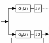
$\displaystyle H_{0}[z] = \frac{1}{\sqrt2} [ 1 + z^{-1} ] $

$\displaystyle H_{1}[z] = \frac{1}{\sqrt2} [ 1 - z^{-1} ] $

Let us look at the frequency response of these filter $\displaystyle H_{0}(w) = \frac{1}{\sqrt2} [ 1 + e^{-j\omega} ] $

$\displaystyle H_{0}(w) = \sqrt{2}e^{-j\frac{\omega}{2}} cos(\frac{\omega}{2}) $

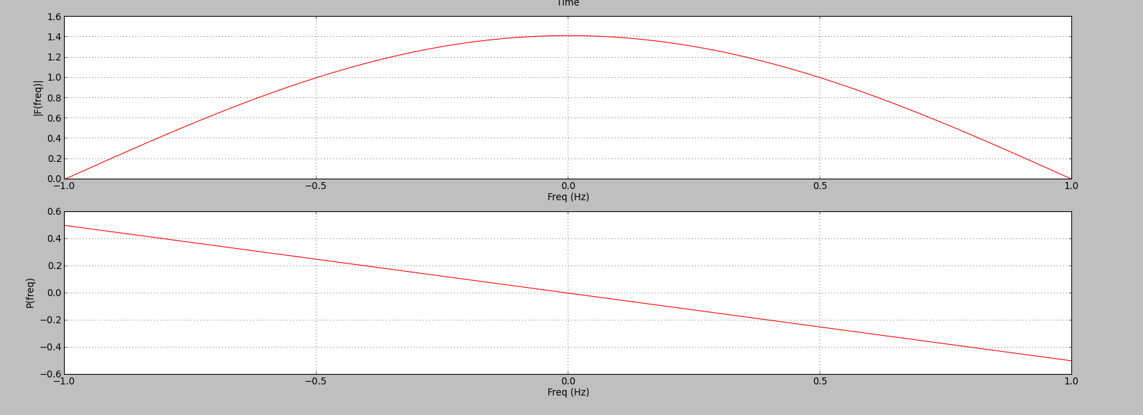
The phase response of the filter is $-\frac{\omega}{2}$ .The filter has linear phase response.

We can see from magnitude response that filter has high gain near 0 frequencies while gain falls to 0 at frequencies near $\omega= \pi$ .This acts like a crude low pass filter

Let us look at the frequency response of these filter $\displaystyle H_{1}(w) = \frac{1}{\sqrt2} [ 1 - e^{-j\omega} ] $

$\displaystyle H_{1}(w) = \sqrt{2}e^{-j\frac{\omega}{2}+\frac{j\pi}{2}} sin(\frac{\omega}{2}) $

We can see from magnitude response that filter has high gain near $\pi$ rads while gain falls to 0 near frequencies of 0 .This acts like a crude high pass filter and also has linear phase of $\frac{\pi}{2} - \frac{\omega}{2}$

we can see that

$\displaystyle

H_{0}(w)

^2 +

H_{1}(w)

^2=1$

we can say that the filters are power complementary

$\displaystyle H_{0}(w) + H_{1}(w)=\sqrt{2}$

Analysis of Reconstruction filter

The reconstruction filter coefficients are given by

$\displaystyle h_{r,l}[n]= \frac{1}{\sqrt2} [ 1 , 1 ] $ or $h_{l}[z] = \frac{1}{\sqrt2}[ 1 + z^{-1}]$

$\displaystyle h_{r,u}[n]= \frac{1}{\sqrt2} [- 1 , 1 ] $ or $h_{u}[z] = \frac{1}{\sqrt2}[ 1- z^{-1}]$

The Haar reconstruction process can be graphically represented as

$\displaystyle G_{0}[z] = \frac{1}{\sqrt2} [ 1 + z^{-1} ] $

$\displaystyle G_{1}[z] = \frac{1}{\sqrt2} [ 1 - z^{-1} ] $

The synthesis filters have identical frequency reponse as corresponding analysis filters . $G_{0}[z] $ represents a crude low pass filter while $G_{1}[z]$ represents a crude high pass filter

Realizable two band filter bank

One question to ask is that if we had used ideal filters would the decomposition and reconstruction still be possible.Instead of using crude filter banks why not use ideal filter banks

We have seen in the article “Discrete Time Fourier Transform for Frequency Analysis” that ideal low pass filter has the infinite impulse response,they are infinitely non causal hence cannot be realized in practice

The filters $H_{0}[z],G_{0}[z]$ aspire to be ideal low pass filter with cutoff frequencies of $\frac{\pi}{2}$

The filters $H_{1}[z],G_{1}[z]$ aspire to be ideal high pass filter with cutoff frequencies of $\frac{\pi}{2}$

They cannot however be ideal filters to be practically realizable ,hence we would want them to be as close to the ideal frequency response as possbile.Have a frequency response close to ideal frequency response and impulse response that is realizable.

The different wavelet families essentially have the decomposition and reconstruction filters that are close to desired ideal frequency response.

Another way to look at the filters is thought the scaling and wavelet functions

$\phi(t)$ is basis of subspace $V_{m-1}$,$\phi(2t)$ defines basis of subspace $V_{m}$ we know that $V_{m-1} \subset V_{m}$,Thus basis of $V_{M-1}$ can be expressed in terms of basis of $V_{m}$

$\displaystyle \phi(t) = [\phi(2t) + \phi(2t -\frac{T}{2})]$

In the earlier article on Haar wavelets we say that $\displaystyle \psi(t) = \phi(t)−\frac{1}{2}\phi(2t−\frac{T}{2}) $

$\displaystyle \psi(t) = \frac{1}{\sqrt{2}}[\phi(2t) - \phi(2t +1)]$

This can be seen from the below figures

Thus the filter coefficients are nothing but the projection coefficients of basis function $\phi(t)$ in $V_{m}$ on subspace $V_{m-1}$ and $W_{m}$ whose basis are defined by set ${\phi(2t)}$

$\displaystyle \phi(t) = \sum_{n} h[n] \phi(2t -n)$ $\displaystyle \psi(t) = \sum_{n} g[n] \phi(2t -n)$

Frequency analysis of wavelet decomposition

The question we ask here is what does wavelet decomposition achieve

we again look at the decomposition filter The decomposition filter coefficients are given by

$\displaystyle h_{d,l}[n]= \frac{1}{\sqrt2} [ 1 , 1 ] $ or $h_{l}[z] = \frac{1}{\sqrt2}[ 1 + z^{-1}]$

$\displaystyle h_{d,u}[n]= \frac{1}{\sqrt2} [- 1 , 1 ] $ or $h_{u}[z] = \frac{1}{\sqrt2}[ 1- z^{-1}]$

The Haar decomposition process can be graphically represented as

$\displaystyle H_{0}[z] = \frac{1}{\sqrt2} [ 1 + z^{-1} ] $

$\displaystyle H_{1}[z] = \frac{1}{\sqrt2} [ 1 - z^{-1} ] $

The first step performed in the decomposition process is low pass and high pass filtering Thus the we are essentially observing the low pass and high pass components idependently

Now we perform downsampling we known that scaling in the time domain leads to expansion in the frequency domain

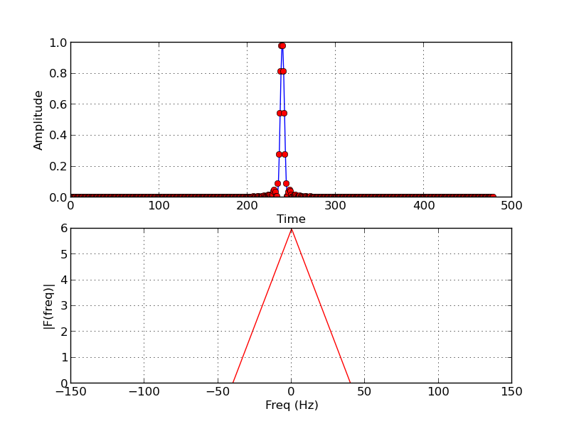
for example let us consider the signal

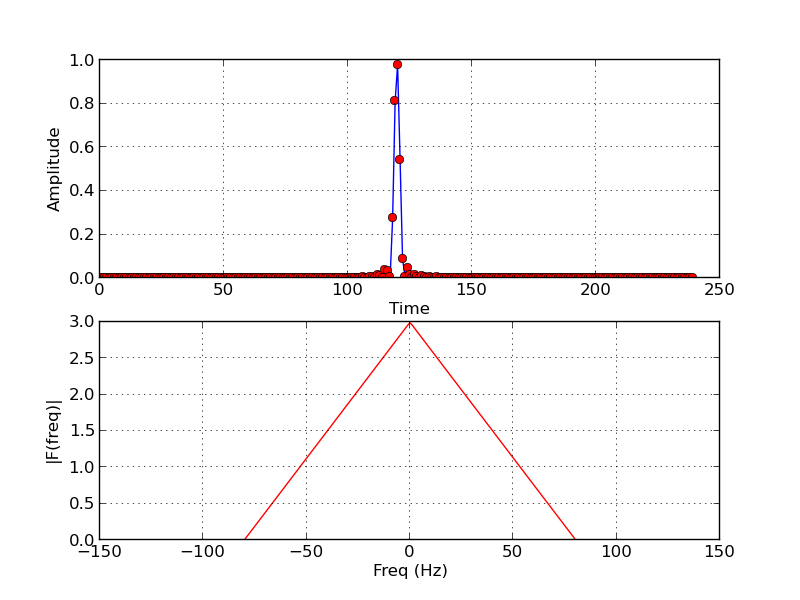
we downsample the signal and observe its frequency response

we can see that original signal had highest frequency content of 40Hz while the downsampled signal has highest frequency content of 80Hz

Thus by dowsampling we have zoomed in on the frequency domain ,while zoomed out in the time domain Thus we have increased the frequency resolution while reduced the time resolution of the signal

Thus by performing decomposition we are first dividing the frequency spectrum of signal into $0-\frac{pi}{2}$ and $\frac{\pi}{2}- \pi$ and zooming in each frequency interval by expanding the $0-\frac{pi}{2}$ interval and $\frac{\pi}{2}- \pi$ interval to $0-pi $ respectively

At the next stage of decompostion,we only consider the output of the low pass filter,which is projection of signal onto $V_{m-1}$ subspace.That is essentially we are looking at the interval $0-\frac{pi}{2}$ of the original signal and again performing the same operation

They by splitting the interval into $0-\frac{pi}{4},\frac{pi}{4}-\frac{pi}{2}$ and so on. Thus at each subspace projection $V_{m-1}$ we are essentially trying to zoom in the frequency domain of the signal while zooming out in the time domain .

Thus we are having a closer look at the frequency spectrum of the signal at each stage of the decomposition.However in standard decompostion process we only zoom into the low pass spectrum of signal. However the same can also be done for high pass spectrum ,ie we want to zoom into the high pass spectrum of the signal.

Another way to look at it is we are succesively dividing the frequency spectrum of the signal at each stage

• Stage 1 - $[0,\frac{\pi}{2}][\frac{\pi}{2},\pi]$

• Stage 2 - $[0,\frac{\pi}{4}][\frac{\pi}{4},\frac{\pi}{2}][\frac{\pi}{2},\pi]$

• Stage 3 - $[0,\frac{\pi}{8}][\frac{\pi}{8},\frac{\pi}{4}][\frac{\pi}{4},\frac{\pi}{2}][\frac{\pi}{2},\pi]$

At each stage we are looking at smaller region in frequency spectrum and conversely large region in the time domain

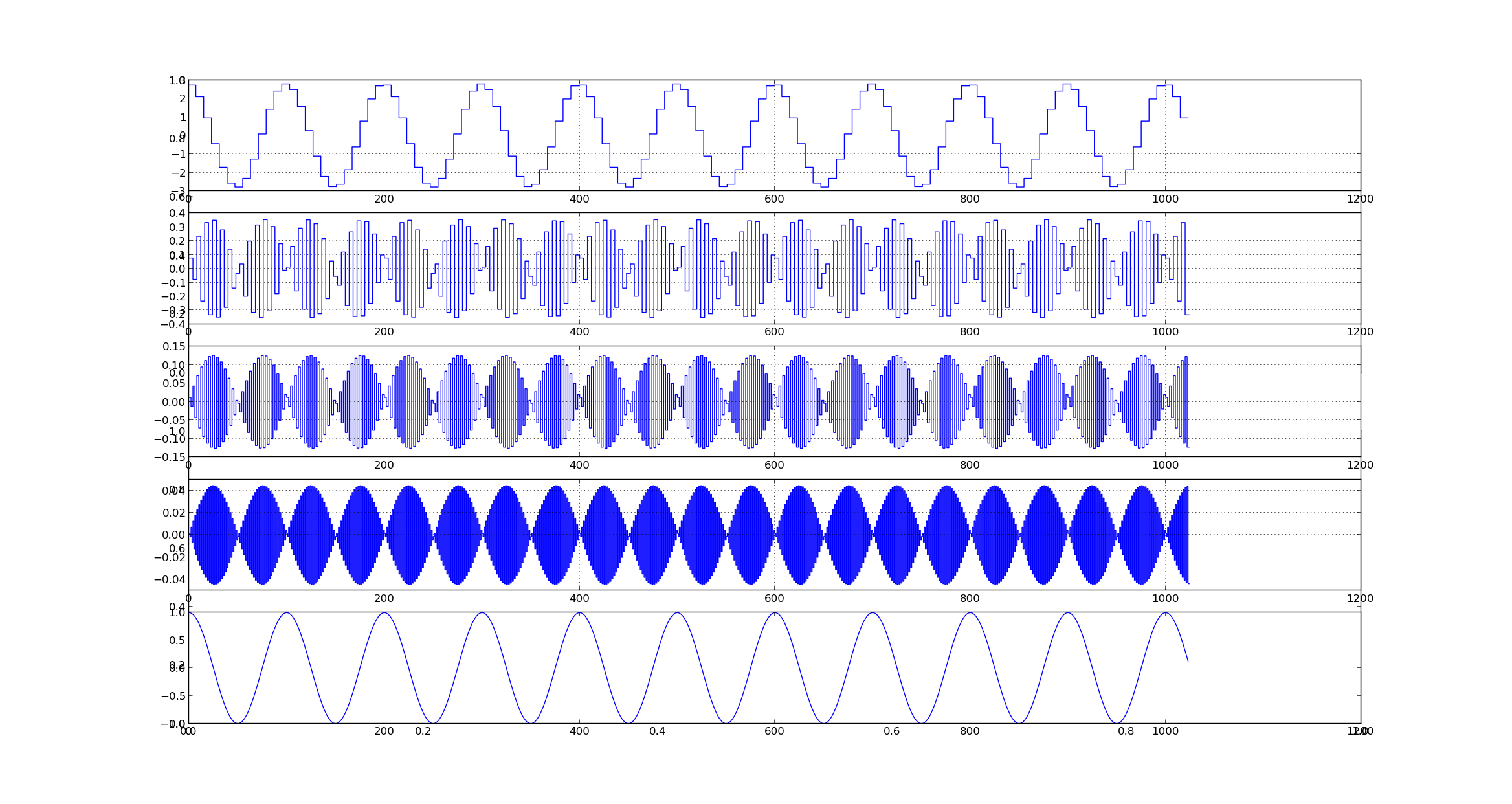
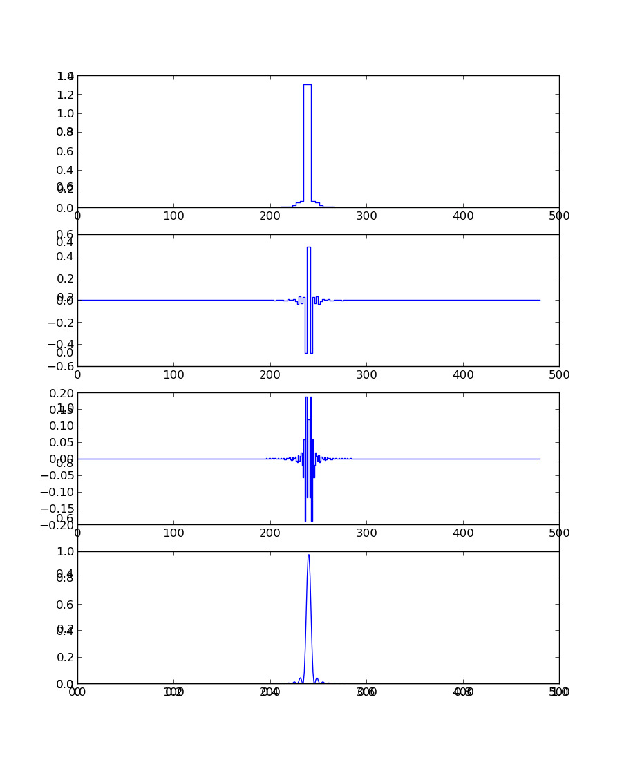
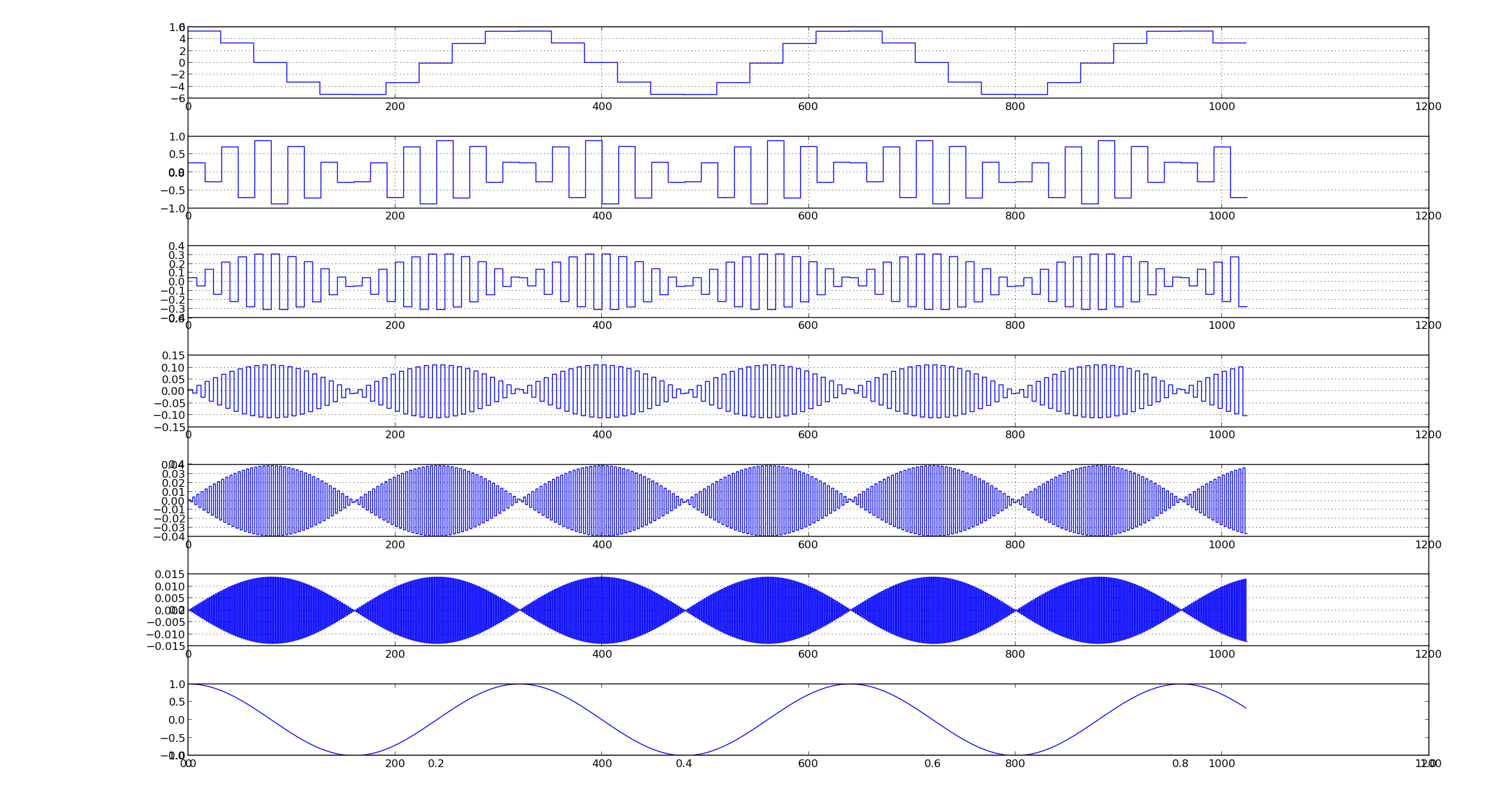
Lets look at the following signal and its decomposition

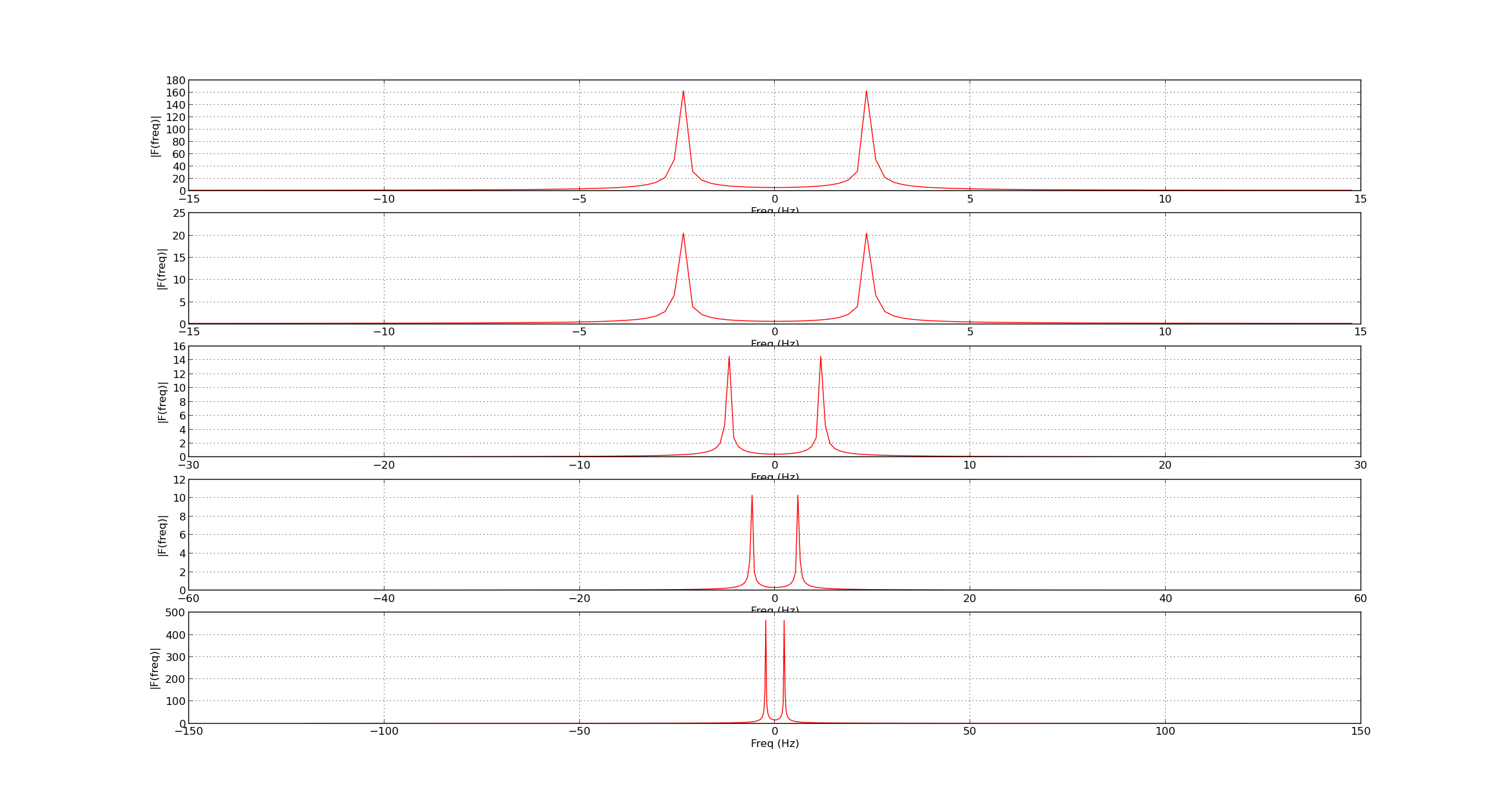
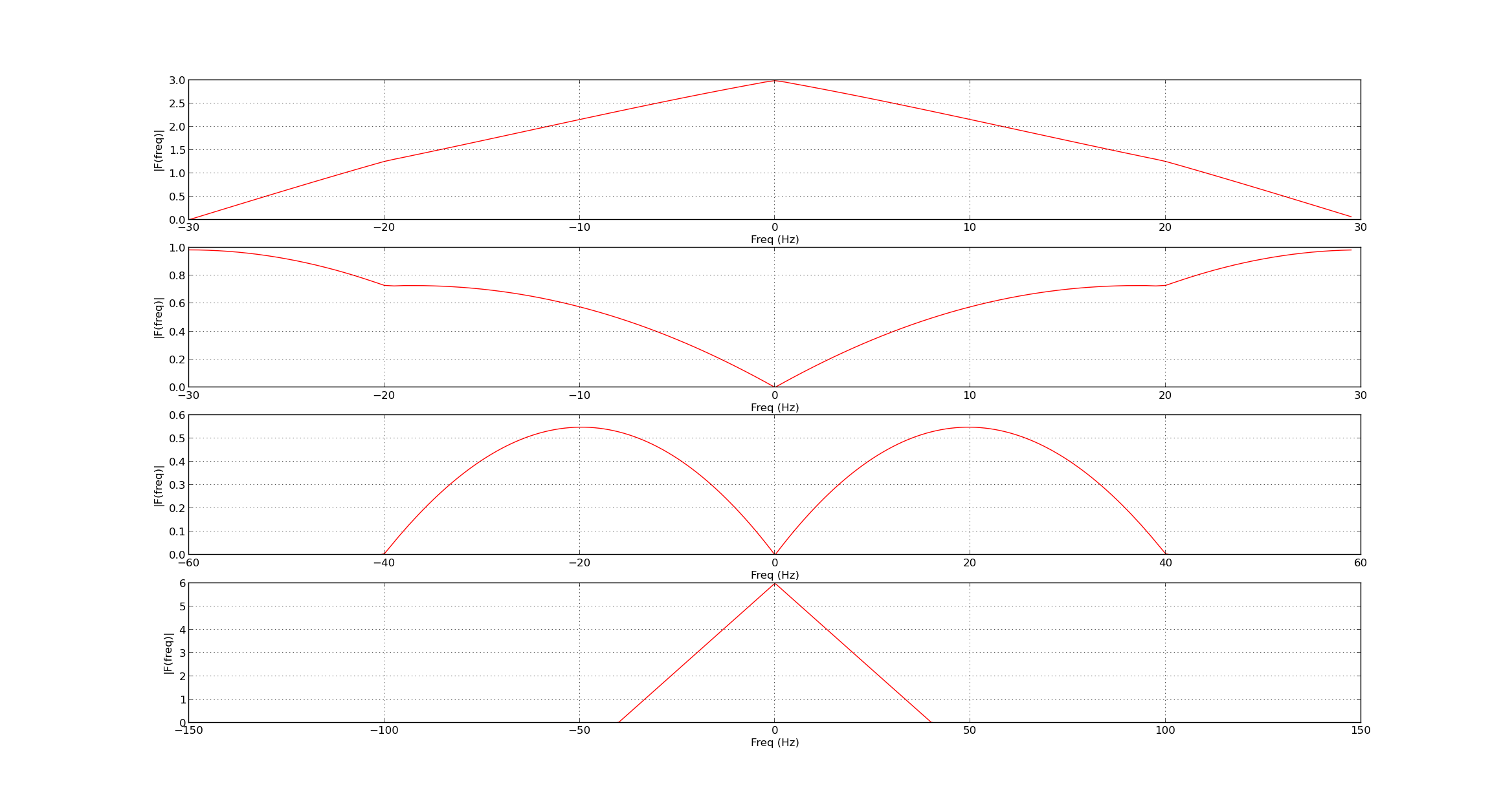
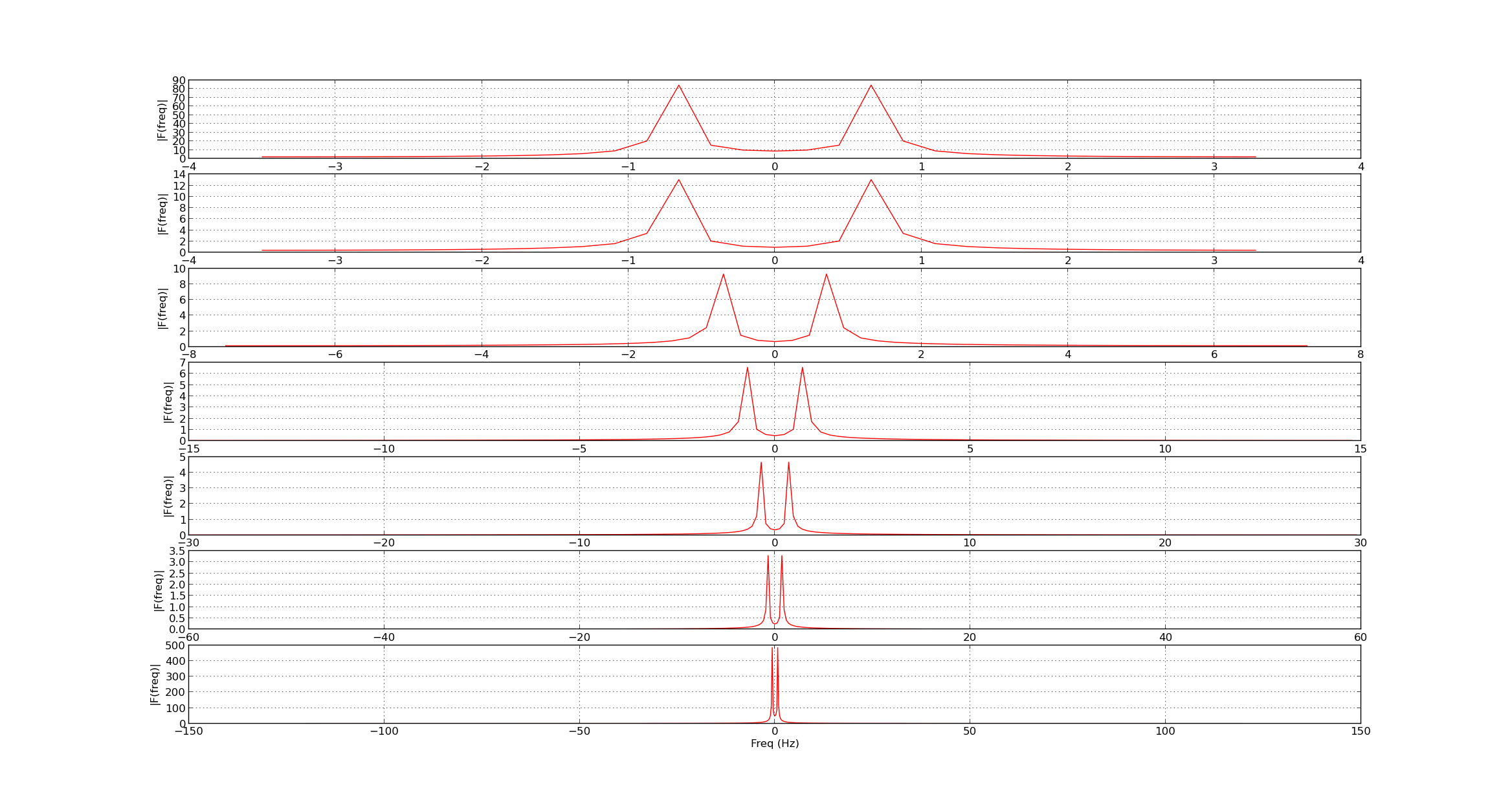
Lets look at the frequency response

We can see piece-wise constant approximation as well as frequency response

The first subplot is the output of the low pass filter or the approximation coefficient of last stage of decomposition and remaining plots are for detail coefficients at each stage of decomposition

we can see that since the filter being used is not ideal low/high pass in decomposition. even though the signal has no high frequency components,the high pass decomposition filter as produced a response.

We can also observe the zooming effect in the frequency response

Below is a plot for sinc squared signal

The same results can be observed for large stages of decomposition

Code

The code for generating all the results and plots can be found the pyVision github repository

• wavelet2.py

running the code

• The code uses pyWavelets python package.This needs to be installed before running the code.
• To run the code,download the entire pyVision repository.
• Go to the pySignalProc/tutorials directory and execute the wavelet2.py code